Neural machine translation with attention
Neural machine translation with attention
Today we shall compose encoder-decoder neural networks and apply them to the task of machine translation.
 (img: esciencegroup.files.wordpress.com)
Encoder-decoder architectures are about converting anything to anything, including
- Machine translation and spoken dialogue systems
- Image captioning and image2latex (convolutional encoder, recurrent decoder)
- Generating images by captions (recurrent encoder, convolutional decoder)
- Grapheme2phoneme - convert words to transcripts
For the neural machine translation project, We will apply first apply a simple encoder-decoder architectute, then we will improve this model with an Attention mecanism.
This post is inspired by a homework from the course NLP For You.
Our task: machine translation
We gonna try our encoder-decoder models on russian to english machine translation problem. More specifically, we’ll translate hotel and hostel descriptions. This task shows the scale of machine translation while not requiring you to train your model for weeks if you don’t use GPU.
Before we get to the architecture, there’s some preprocessing to be done. Go tokenize Alright, this time we’ve done preprocessing for you. As usual, the data will be tokenized with WordPunctTokenizer.
However, there’s one more thing to do. Our data lines contain unique rare words. If we operate on a word level, we will have to deal with large vocabulary size. If instead we use character-level models, it would take lots of iterations to process a sequence. This time we’re gonna pick something inbetween.
One popular approach is called Byte Pair Encoding aka BPE. The algorithm starts with a character-level tokenization and then iteratively merges most frequent pairs for N iterations. This results in frequent words being merged into a single token and rare words split into syllables or even characters.
#!pip3 install tensorflow-gpu>=2.0.0
#!pip3 install subword-nmt &> log
# !wget https://www.dropbox.com/s/yy2zqh34dyhv07i/data.txt?dl=1 -O data.txt
# !wget https://www.dropbox.com/s/fj9w01embfxvtw1/dummy_checkpoint.npz?dl=1 -O dummy_checkpoint.npz
# !wget https://raw.githubusercontent.com/yandexdataschool/nlp_course/2019/week04_seq2seq/utils.py -O utils.py
# thanks to tilda and deephack teams for the data, Dmitry Emelyanenko for the code :)
from nltk.tokenize import WordPunctTokenizer
from subword_nmt.learn_bpe import learn_bpe
from subword_nmt.apply_bpe import BPE
tokenizer = WordPunctTokenizer()
def tokenize(x):
    return ' '.join(tokenizer.tokenize(x.lower()))

# split and tokenize the data
with open('train.en', 'w', encoding="utf8") as f_src,  open('train.ru', 'w', encoding="utf8") as f_dst:
    for line in open('data.txt', encoding="utf8"):
        src_line, dst_line = line.strip().split('\t')
        f_src.write(tokenize(src_line) + '\n')
        f_dst.write(tokenize(dst_line) + '\n')

# build and apply bpe vocs
bpe = {}
for lang in ['en', 'ru']:
    learn_bpe(open('./train.' + lang, encoding="utf8"), open('bpe_rules.' + lang, 'w', encoding="utf8"), num_symbols=8000)
    bpe[lang] = BPE(open('./bpe_rules.' + lang, encoding="utf8"))

    with open('train.bpe.' + lang, 'w', encoding="utf8") as f_out:
        for line in open('train.' + lang, encoding="utf8"):
            f_out.write(bpe[lang].process_line(line.strip()) + '\n')
Building vocabularies
We now need to build vocabularies that map strings to token ids and vice versa. We’re gonna need these fellas when we feed training data into model or convert output matrices into words.
import numpy as np
import matplotlib.pyplot as plt
%matplotlib inline
data_inp = np.array(open('./train.bpe.ru', encoding="utf8").read().split('\n'))
data_out = np.array(open('./train.bpe.en', encoding="utf8").read().split('\n'))

from sklearn.model_selection import train_test_split
train_inp, dev_inp, train_out, dev_out = train_test_split(data_inp, data_out, test_size=3000,
                                                          random_state=42)
for i in range(3):
    print('inp:', train_inp[i])
    print('out:', train_out[i], end='\n\n')
from utils import Vocab
inp_voc = Vocab.from_lines(train_inp)
out_voc = Vocab.from_lines(train_out)
# Here's how you cast lines into ids and backwards.
batch_lines = sorted(train_inp, key=len)[5:10]
batch_ids = inp_voc.to_matrix(batch_lines)
batch_lines_restored = inp_voc.to_lines(batch_ids)

print("lines")
print(batch_lines)
print("\nwords to ids (0 = bos, 1 = eos):")
print(batch_ids)
print("\nback to words")
print(batch_lines_restored)
Draw source and translation length distributions to estimate the scope of the task.
plt.figure(figsize=[8, 4])
plt.subplot(1, 2, 1)
plt.title("source length")
plt.hist(list(map(len, map(str.split, train_inp))), bins=20);

plt.subplot(1, 2, 2)
plt.title("translation length")
plt.hist(list(map(len, map(str.split, train_out))), bins=20);
Encoder-decoder model
The code below contains a template for a simple encoder-decoder model: single GRU encoder/decoder, no attention or anything.
import tensorflow as tf
assert tf.__version__.startswith('2'), "Current tf version: {}; required: 2.0.*".format(tf.__version__)
L = tf.keras.layers
keras = tf.keras
from utils import infer_length, infer_mask
class BasicModel(L.Layer):
    def __init__(self, inp_voc, out_voc, emb_size=64, hid_size=128):
        """
        A simple encoder-decoder model
        """
        super().__init__() # initialize base class to track sub-layers, trainable variables, etc.

        self.inp_voc, self.out_voc = inp_voc, out_voc
        self.hid_size = hid_size

        self.emb_inp = L.Embedding(len(inp_voc), emb_size)
        self.emb_out = L.Embedding(len(out_voc), emb_size)
        self.enc0 = L.GRUCell(hid_size)

        self.dec_start = L.Dense(hid_size)
        self.dec0 = L.GRUCell(hid_size)
        self.logits = L.Dense(len(out_voc))

    def encode(self, inp, **flags):
        """
        Takes symbolic input sequence, computes initial state
        :param inp: matrix of input tokens [batch, time]
        :returns: initial decoder state tensors, one or many
        """
        inp_emb = self.emb_inp(inp)
        batch_size = inp.shape[0]

        mask = infer_mask(inp, self.inp_voc.eos_ix, dtype=tf.bool)

        state = [tf.zeros((batch_size, self.hid_size), tf.float32)]

        for i in tf.range(inp_emb.shape[1]):
            output, next_state = self.enc0(inp_emb[:, i], state)
            state = [
                     tf.where(
                         tf.tile(mask[:, i, None],[1,next_tensor.shape[1]]),
                         next_tensor, tensor
                      ) for tensor, next_tensor in zip(state, next_state)
            ]

        dec_start = self.dec_start(state[0])
        return [dec_start]

    def decode_step(self, prev_state, prev_tokens, **flags):
        """
        Takes previous decoder state and tokens, returns new state and logits for next tokens
        :param prev_state: a list of previous decoder state tensors
        :param prev_tokens: previous output tokens, an int vector of [batch_size]
        :return: a list of next decoder state tensors, a tensor of logits [batch, n_tokens]
        """
        out_emb = self.emb_inp(prev_tokens)

        output_dec, new_dec_state = self.dec0(out_emb, prev_state)
        output_logits = self.logits(output_dec)
        return new_dec_state, output_logits

    def decode(self, initial_state, out_tokens, **flags):
        """ Run decoder on reference tokens (out_tokens) """
        state = initial_state
        batch_size = out_tokens.shape[0]

        # initial logits: always predict BOS
        first_logits = tf.math.log(
            tf.one_hot(tf.fill([batch_size], self.out_voc.bos_ix), len(self.out_voc)) + 1e-30)
        outputs = [first_logits]

        for i in tf.range(out_tokens.shape[1] - 1):
            state, logits = self.decode_step(state, out_tokens[:, i])
            outputs.append(logits)

        return tf.stack(outputs, axis=1)

    def call(self, inp, out):
        """ Apply model in training mode """
        initial_state = self.encode(inp)
        return self.decode(initial_state, out)

    def decode_inference(self, initial_state, max_len=100, **flags):
        """ Generate translations from model (greedy version) """
        state = initial_state
        outputs = [tf.ones(initial_state[0].shape[0], tf.int32) * self.out_voc.bos_ix]
        all_states = [initial_state]

        for i in tf.range(max_len):
            state, logits = self.decode_step(state, outputs[-1])
            outputs.append(tf.argmax(logits, axis=-1, output_type=tf.int32))
            all_states.append(state)

        return tf.stack(outputs, axis=1), all_states

    def translate_lines(self, inp_lines):
        inp = tf.convert_to_tensor(inp_voc.to_matrix(inp_lines))

        initial_state = self.encode(inp)
        out_ids, states = self.decode_inference(initial_state)
        return out_voc.to_lines(out_ids.numpy()), states
model = BasicModel(inp_voc, out_voc)
dummy_inp = tf.convert_to_tensor(inp_voc.to_matrix(train_inp[:3]))
dummy_out = tf.convert_to_tensor(out_voc.to_matrix(train_out[:3]))
dummy_logits = model(dummy_inp, dummy_out)
ref_shape = (dummy_out.shape[0], dummy_out.shape[1], len(out_voc))
assert dummy_logits.shape == ref_shape, "Your logits shape should be {} but got {}".format(dummy_logits.shape, ref_shape)
assert all(dummy_logits[:, 0].numpy().argmax(-1) == out_voc.bos_ix), "first step must always be BOS"
Training loss
Our training objective is almost the same as it was for neural language models: \(L = {\frac1{|D|}} \sum_{X, Y \in D} \sum_{y_t \in Y} - \log p(y_t \mid y_1, \dots, y_{t-1}, X, \theta)\)
where \(|D|\) is the total length of all sequences, including BOS and first EOS, but excluding PAD.
def compute_loss(model, inp, out, **flags):
    """
    Compute loss (float32 scalar) as in the formula above
    :param inp: input tokens matrix, int32[batch, time]
    :param out: reference tokens matrix, int32[batch, time]

    In order to pass the tests, your function should
    * include loss at first EOS but not the subsequent ones
    * divide sum of losses by a sum of input lengths (use infer_length or infer_mask)
    """
    inp, out = map(tf.convert_to_tensor, [inp, out])
    targets_1hot = tf.one_hot(out, len(model.out_voc), dtype=tf.float32)
    mask = infer_mask(out, out_voc.eos_ix) # [batch_size, out_len]

    # outputs of the model, [batch_size, out_len, num_tokens]
    logits_seq = model(inp, out)

    # log-probabilities of all tokens at all steps, [batch_size, out_len, num_tokens]
    #print(logprobs_seq.shape)
    logprobs_seq = -tf.math.maximum(tf.math.log(tf.nn.softmax(logits_seq)), tf.math.log(2**-30))
    #print(logprobs_seq.shape)
    # log-probabilities of correct outputs, [batch_size, out_len]
    logp_out = tf.reduce_sum(logprobs_seq * targets_1hot, axis=-1)
    #print(logp_out.shape)
    # mean cross-entropy over tokens where mask == 1
    return tf.reduce_sum(logp_out * mask)/tf.cast(tf.reduce_sum(infer_length(inp, inp_voc.eos_ix)), tf.float32) # scalar
dummy_loss = compute_loss(model, dummy_inp, dummy_out)
print("Loss:", dummy_loss)
assert np.allclose(dummy_loss, 8.425, rtol=0.1, atol=0.1), "We're sorry for your loss"
Evaluation: BLEU
Machine translation is commonly evaluated with BLEU score. This metric simply computes which fraction of predicted n-grams is actually present in the reference translation. It does so for n=1,2,3 and 4 and computes the geometric average with penalty if translation is shorter than reference.
While BLEU has many drawbacks, it still remains the most commonly used metric and one of the simplest to compute.
from nltk.translate.bleu_score import corpus_bleu
def compute_bleu(model, inp_lines, out_lines, bpe_sep='@@ ', **flags):
    """
    Estimates corpora-level BLEU score of model's translations given inp and reference out
    Note: if you're serious about reporting your results, use https://pypi.org/project/sacrebleu
    """
    translations, _ = model.translate_lines(inp_lines, **flags)
    translations = [line.replace(bpe_sep, '') for line in translations]
    return corpus_bleu(
        [[ref.split()] for ref in out_lines],
        [trans.split() for trans in translations],
        smoothing_function=lambda precisions, **kw: [p + 1.0 / p.denominator for p in precisions]
        ) * 100
compute_bleu(model, dev_inp, dev_out)
Training loop
Training encoder-decoder models isn’t that different from any other models: sample batches, compute loss, backprop and update.
from IPython.display import clear_output
from tqdm import tqdm, trange
metrics = {'train_loss': [], 'dev_bleu': [] }

opt = keras.optimizers.Adam(1e-3)
batch_size = 32
for _ in trange(25000):
    step = len(metrics['train_loss']) + 1
    batch_ix = np.random.randint(len(train_inp), size=batch_size)
    batch_inp = inp_voc.to_matrix(train_inp[batch_ix])
    batch_out = out_voc.to_matrix(train_out[batch_ix])

    with tf.GradientTape() as tape:
         loss_t = compute_loss(model, batch_inp, batch_out)

    grads = tape.gradient(loss_t, model.trainable_variables)
    opt.apply_gradients(zip(grads, model.trainable_variables))


    metrics['train_loss'].append((step, loss_t.numpy()))

    if step % 100 == 0:
        metrics['dev_bleu'].append((step, compute_bleu(model, dev_inp, dev_out)))

        clear_output(True)
        plt.figure(figsize=(12,4))
        for i, (name, history) in enumerate(sorted(metrics.items())):
            plt.subplot(1, len(metrics), i + 1)
            plt.title(name)
            plt.plot(*zip(*history))
            plt.grid()
        plt.show()
        print("Mean loss=%.3f" % np.mean(metrics['train_loss'][-10:], axis=0)[1], flush=True)

# Note: it's okay if bleu oscillates up and down as long as it gets better on average over long term (e.g. 5k batches)
assert np.mean(metrics['dev_bleu'][-10:], axis=0)[1] > 15, "We kind of need a higher bleu BLEU from you. Kind of
 right now."
Here are the outputs from the training step:
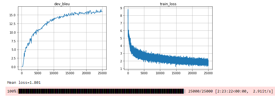
We see that there is convergence for the loss function. And at the end of the training the blue metric is above 15.
for inp_line, trans_line in zip(dev_inp[::500], model.translate_lines(dev_inp[::500])[0]):
    print(inp_line)
    print(trans_line)
    print()
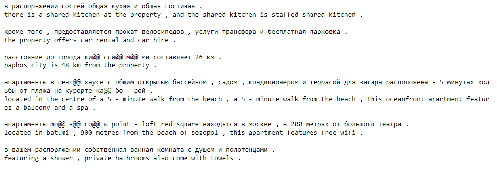
The screenshot above shows a few translations from the validation set.
We can still spot some obvious mistakes:
- For instance for the first translation, the part the shared kitchen is staffed shared kitchen doesn’t mean anything
- For the 3rd sentence 26 KM is translated by 48 KM
But overral, the result is not so bad. Can we do better ?
Network Machine Translation (NMT) with Attention
Your Attention Required
In this section we want you to improve over the basic model by implementing a simple attention mechanism.
This is gonna be a two-parter: building the attention layer and using it for an attentive seq2seq model.
Attention layer
Here you will have to implement a layer that computes a simple additive attention:
Given encoder sequence \(h^e_0, h^e_1, h^e_2, ..., h^e_T\) and a single decoder state \(h^d\),
- Compute logits with a 2-layer neural network \(a_t = linear_{out}(tanh(linear_{e}(h^e_t) + linear_{d}(h_d)))\)
-
Get probabilities from logits,
\(p_t\) = \({e ^ {a_t}} \over { \sum_\tau e^{a_\tau} }\) - Add up encoder states with probabilities to get attention response
\(attn = \sum_t p_t \cdot h^e_t\)
You can learn more about attention layers in the lecture slides or from this post.
class AttentionLayer(L.Layer):
    def __init__(self, name, enc_size, dec_size, hid_size, activ=tf.tanh):
        """ A layer that computes additive attention response and weights """
        super().__init__()
        self._name = name
        self.enc_size = enc_size # num units in encoder state
        self.dec_size = dec_size # num units in decoder state
        self.hid_size = hid_size # attention layer hidden units
        self.activ = activ       # attention layer hidden nonlinearity

    def build(self, input_shape):
        # create layer variables
        self.e_w = self.add_weight("enc_weight", shape=[int(input_shape[-1]), self.hid_size])
        self.d_w = self.add_weight("dec_weight", shape=[int(input_shape[-1]), self.hid_size])
        self.o_w = self.add_weight("out_weight", shape=[self.hid_size, 1])


        # Hint: you can find an example of custom layer here:
        # https://www.tensorflow.org/tutorials/customization/custom_layers

    def call(self, enc, dec, inp_mask):
        """
        Computes attention response and weights
        :param enc: encoder activation sequence, float32[batch_size, ninp, enc_size]
        :param dec: single decoder state used as "query", float32[batch_size, dec_size]
        :param inp_mask: mask on enc activations (0 after first eos), float32 [batch_size, ninp]
        :returns: attn[batch_size, enc_size], probs[batch_size, ninp]
            - attn - attention response vector (weighted sum of enc)
            - probs - attention weights after softmax
        """

        # Compute logits
        #<...>
        #logits = []
#         print("self.e_w :", self.e_w.shape)
#         print("self.d_w :", self.d_w.shape)
        # Add time dimension to decode input to be able to sum with encode input
        dec_with_time = tf.expand_dims(dec, 1)
        logits = tf.matmul(self.activ(tf.matmul(enc, self.e_w) + tf.matmul(dec_with_time, self.d_w)), self.o_w)


        # Apply mask - if mask is 0, logits should be -inf or -1e9
        # You may need tf.where
        #<...>
        #logits *= inp_mask
        lower_cap = -1e9 * tf.ones_like(logits)
        #print("inp_mask: ", inp_mask)
        logits = tf.where(tf.expand_dims(inp_mask, -1), logits, lower_cap )
        #print(logits)

        # Compute attention probabilities (softmax)
        # Sum of probs must be 1 along axis 1
        probs = tf.nn.softmax(logits, axis=1)
        #print("probs: ", probs.shape)

        # Compute attention response using enc and probs
        #print("enc: ", enc.shape)
        attn = probs * enc
        #print("attn: ", attn.shape)
        attn = tf.reduce_sum(attn, axis = 1)
        #print("attn: ", attn.shape)
        probs = tf.reshape(probs, [inp_mask.shape[0],-1])
        #print("probs: ", probs.shape)

        return attn, probs
# Test the attention layer
layer = AttentionLayer('JL attention layer', 64, 64, 128)
_ = layer(tf.ones([3,25, 128]), tf.ones([3, 128]), tf.ones([3,25], tf.bool))
print([var.name for var in layer.trainable_variables])
Seq2seq model with attention
You can now use the attention layer to build a network. The simplest way to implement attention is to use it in decoder phase:
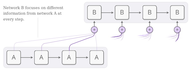 image from distill.pub article
On every step, use previous decoder state to obtain attention response. Then feed concat this response to the inputs of next attention layer of the next decoder step:
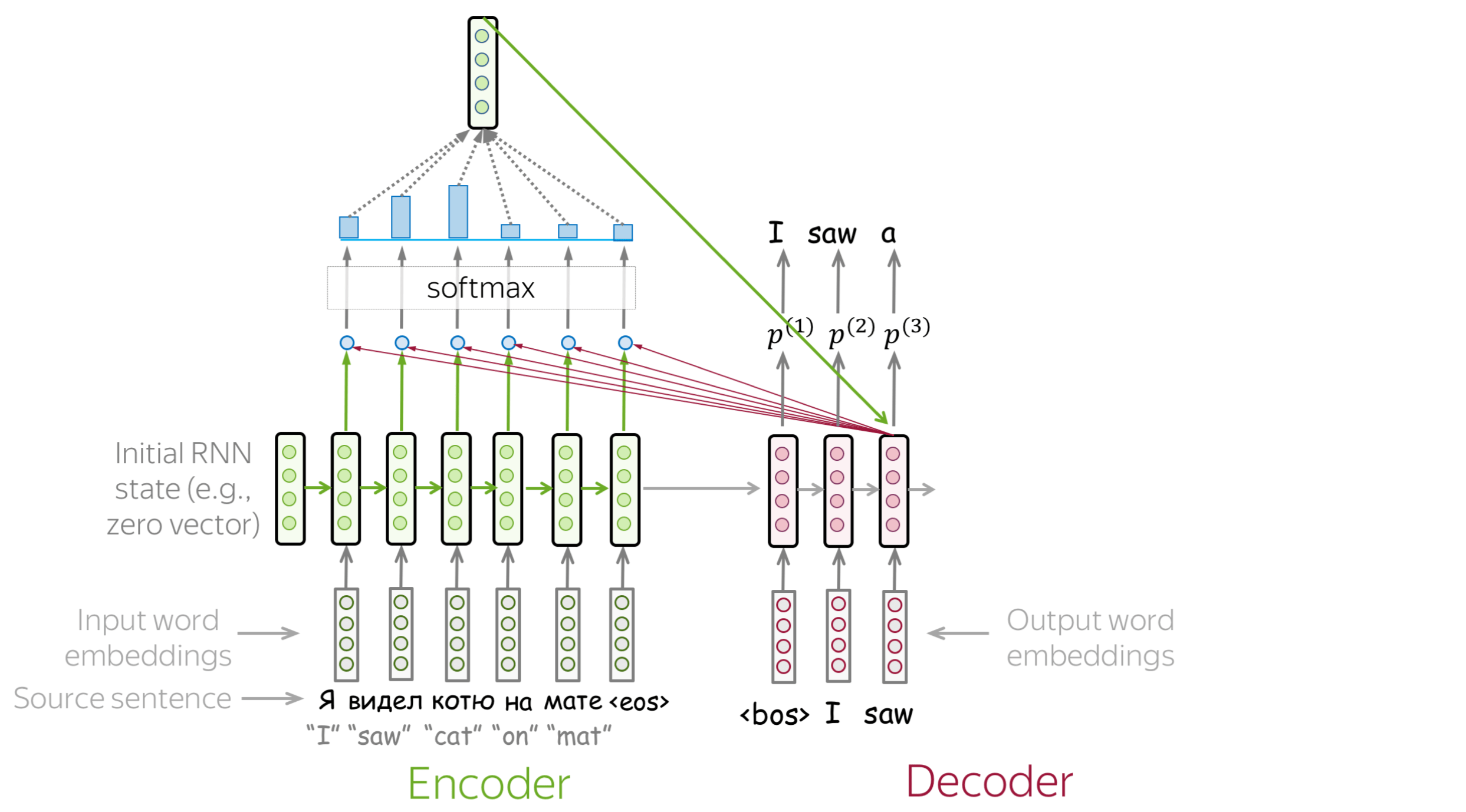
The key implementation detail here is model state. Put simply, you can add any tensor into the list of encode outputs. You will then have access to them at each decode step. This may include:
- Last RNN hidden states (as in basic model)
- The whole sequence of encoder outputs (to attend to) and mask
- Attention probabilities (to visualize)
- Attention values (context)
There are, of course, alternative ways to wire attention into your network and different kinds of attention. Take a look at this, this and this for ideas. And for image captioning/im2latex there’s visual attention
class AttentiveModel(BasicModel):
    def __init__(self, name, inp_voc, out_voc,
                 emb_size=64, hid_size=128, attn_size=128):
        """ Translation model that uses attention. See instructions above. """
        L.Layer.__init__(self) # initialize base class to track sub-layers, trainable variables, etc.

        self.inp_voc, self.out_voc = inp_voc, out_voc
        self.hid_size = hid_size

        #<initialize layers>
        self._name = name
        self.emb_inp = L.Embedding(len(inp_voc), emb_size)
        self.emb_out = L.Embedding(len(out_voc), emb_size)
        # Encocoding GRU cell
        self.enc0 = L.GRUCell(hid_size)

        # Decoding Start Layer
        self.dec_start = L.Dense(hid_size)
        # Decoding GRU cell
        self.dec0 = L.GRUCell(hid_size)

        # Attention layer
        self.attn = AttentionLayer("attnLayer", len(inp_voc), len(out_voc), attn_size)
        # Logits layer
        self.logits = L.Dense(len(out_voc))

    def encode(self, inp, **flags):
        """
        Takes symbolic input sequence, computes initial state
        :param inp: matrix of input tokens [batch, time]
        :return: a list of initial decoder state tensors
        """

        # encode input sequence, create initial decoder states
        #
        inp_emb = self.emb_inp(inp)
        batch_size = inp.shape[0]

        mask = infer_mask(inp, self.inp_voc.eos_ix, dtype=tf.bool)

        state = [tf.zeros((batch_size, self.hid_size), tf.float32)]
        outputs = []
        for i in tf.range(inp_emb.shape[1]):
            output, next_state = self.enc0(inp_emb[:, i], state)
            outputs.append(output)
            state = [
                     tf.where(
                         tf.tile(mask[:, i, None],[1,next_tensor.shape[1]]),
                         next_tensor, tensor
                      ) for tensor, next_tensor in zip(state, next_state)
            ]
        # To be used by the decoding network
        dec_start = self.dec_start(state[0])
        # Full output from the encoding network: Will be used by the Attention layer
        outputs = tf.stack(outputs, axis = 1)
        # apply attention layer from initial decoder hidden state
        attn_val, first_attn_probas = self.attn(outputs, dec_start, mask)
        # Build first state: include
        # * initial states for decoder recurrent layers
        # * encoder sequence and encoder attn mask (for attention)
        # * attn_val (i.e. context)
        # * make sure that last state item is attention probabilities tensor

        # First state will be used by the decoder network
        first_state = [dec_start, outputs, mask, attn_val, first_attn_probas]
        return first_state

    def decode_step(self, prev_state, prev_tokens, **flags):
        """
        Takes previous decoder state and tokens, returns new state and logits for next tokens
        :param prev_state: a list of previous decoder state tensors
        :param prev_tokens: previous output tokens, an int vector of [batch_size]
        :return: a list of next decoder state tensors, a tensor of logits [batch, n_tokens]
        """

        #
        # Apply output (decoding) embedding
        out_emb = self.emb_out(prev_tokens)
        # Get Attention value (context) from previous state
        attn_val = prev_state[3]
        # Concat embedding with attention context
        out_emb = tf.concat([out_emb, attn_val], axis = -1)
        # Apply decoding cell to attention concatenated embedding and previous state to get output_decoding and new state
        output_dec, dec_state = self.dec0(out_emb, prev_state)
        # Apply the fully connected layer to get the logits
        output_logits = self.logits(output_dec)
        # Apply the attention layer to the new output from decoding cell (output_dec)
        # We use prev_state[1] (encoder output) and prev_state[2] (mask)
        attn_val, attn_prob = self.attn(prev_state[1], output_dec, prev_state[2])
        # we store the attn_val and attn_prob in the new_dec_state
        new_dec_state = [dec_state[0], prev_state[1], prev_state[2],  attn_val, attn_prob]
        return new_dec_state, output_logits
model = AttentiveModel("AttentionModel", inp_voc, out_voc)
dummy_inp = tf.convert_to_tensor(inp_voc.to_matrix(train_inp[:3]))
dummy_out = tf.convert_to_tensor(out_voc.to_matrix(train_out[:3]))
dummy_logits = model(dummy_inp, dummy_out)
ref_shape = (dummy_out.shape[0], dummy_out.shape[1], len(out_voc))
assert dummy_logits.shape == ref_shape, "Your logits shape should be {} but got {}".format(dummy_logits.shape, ref_shape)
assert all(dummy_logits[:, 0].numpy().argmax(-1) == out_voc.bos_ix), "first step must always be BOS"
Training attentive model
We will reuse the infrastructure we’ve built for the regular model.
#<create AttentiveModel and training utilities>
model = AttentiveModel("AttentionModel", inp_voc, out_voc)
#<training loop>
for _ in trange(25000):
    step = len(metrics['train_loss']) + 1
    batch_ix = np.random.randint(len(train_inp), size=batch_size)
    batch_inp = inp_voc.to_matrix(train_inp[batch_ix])
    batch_out = out_voc.to_matrix(train_out[batch_ix])

    with tf.GradientTape() as tape:
         loss_t = compute_loss(model, batch_inp, batch_out)

    grads = tape.gradient(loss_t, model.trainable_variables)
    opt.apply_gradients(zip(grads, model.trainable_variables))


    metrics['train_loss'].append((step, loss_t.numpy()))

    if step % 100 == 0:
        metrics['dev_bleu'].append((step, compute_bleu(model, dev_inp, dev_out)))

        clear_output(True)
        plt.figure(figsize=(12,4))
        for i, (name, history) in enumerate(sorted(metrics.items())):
            plt.subplot(1, len(metrics), i + 1)
            plt.title(name)
            plt.plot(*zip(*history))
            plt.grid()
        plt.show()
        print("Mean loss=%.3f" % np.mean(metrics['train_loss'][-10:], axis=0)[1], flush=True)
Here are the outputs from the training step:
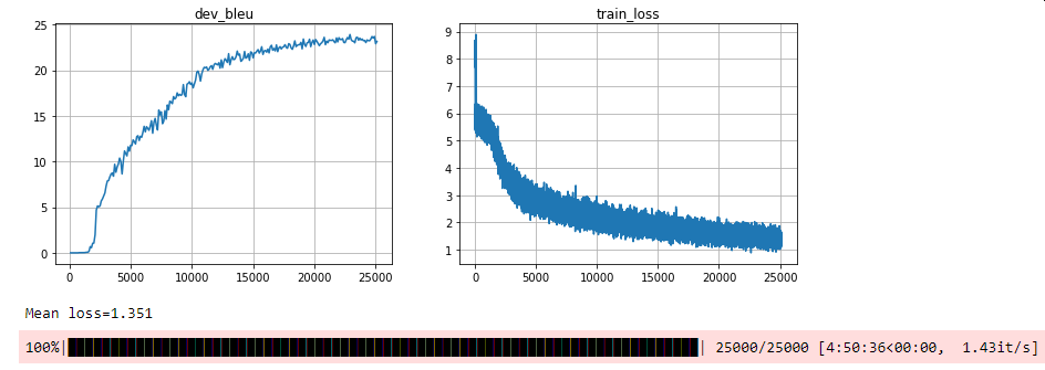
We see that the loss converged, and that the blue metric is above 23 (to be compared to 15 for the base model).
Therefore we have a better model. Let’s check with a few samples.
for inp_line, trans_line in zip(dev_inp[::500], model.translate_lines(dev_inp[::500])[0]):
    print(inp_line)
    print(trans_line)
    print()
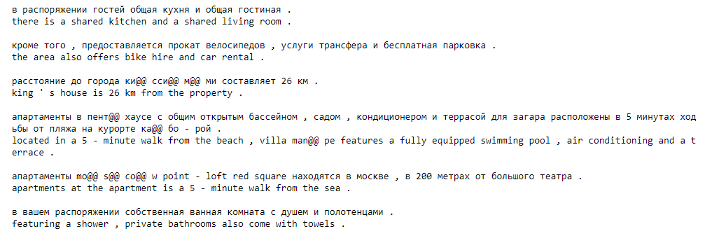 Here all the English sentences generated seems to be correct. There is no big obvious mistakes like with the base model.
Visualizing model attention
After training the attentive translation model, you can check it’s sanity by visualizing its attention weights.
We provided you with a function that draws attention maps using Bokeh.
import bokeh.plotting as pl
import bokeh.models as bm
from bokeh.io import output_notebook, show
output_notebook()

def draw_attention(inp_line, translation, probs):
    """ An intentionally ambiguous function to visualize attention weights """
    inp_tokens = inp_voc.tokenize(inp_line)
    trans_tokens = out_voc.tokenize(translation)
    probs = probs[:len(trans_tokens), :len(inp_tokens)]

    fig = pl.figure(x_range=(0, len(inp_tokens)), y_range=(0, len(trans_tokens)),
                    x_axis_type=None, y_axis_type=None, tools=[])
    fig.image([probs[::-1]], 0, 0, len(inp_tokens), len(trans_tokens))

    fig.add_layout(bm.LinearAxis(axis_label='source tokens'), 'above')
    fig.xaxis.ticker = np.arange(len(inp_tokens)) + 0.5
    fig.xaxis.major_label_overrides = dict(zip(np.arange(len(inp_tokens)) + 0.5, inp_tokens))
    fig.xaxis.major_label_orientation = 45

    fig.add_layout(bm.LinearAxis(axis_label='translation tokens'), 'left')
    fig.yaxis.ticker = np.arange(len(trans_tokens)) + 0.5
    fig.yaxis.major_label_overrides = dict(zip(np.arange(len(trans_tokens)) + 0.5, trans_tokens[::-1]))

    show(fig, notebook_handle = True)
inp = dev_inp[::500]

trans, states = model.translate_lines(inp)
# for state in states:
#     print("state : ", state[-1].shape)

# select attention probs from model state (you may need to change this for your custom model)
# attention_probs below must have shape [batch_size, translation_length, input_length], extracted from states
# e.g. if attention probs are at the end of each state, use np.stack([state[-1] for state in states], axis=1)
attention_probs = np.stack([state[-1]  for i,state in enumerate(states)], axis=1)
for i in range(5):
    draw_attention(inp[i], trans[i], attention_probs[i])
Here are the attention probabilities for the 5 samples:
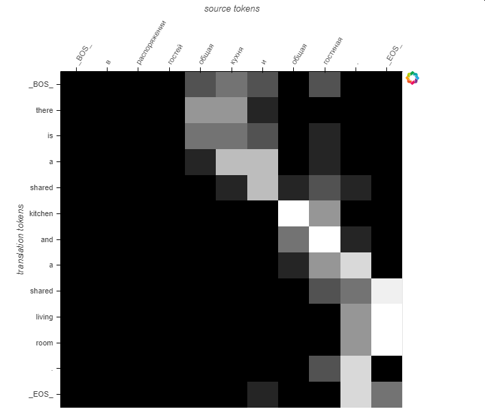 We see that the attention probabilities follow the diagonal but seems to be shifted to the right.
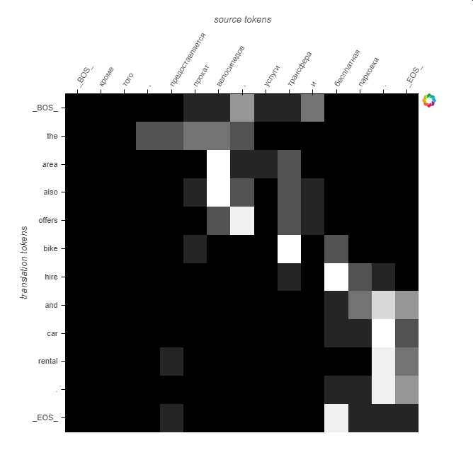 We see the same pattern as with sample 1, but the word the has a larger scope.
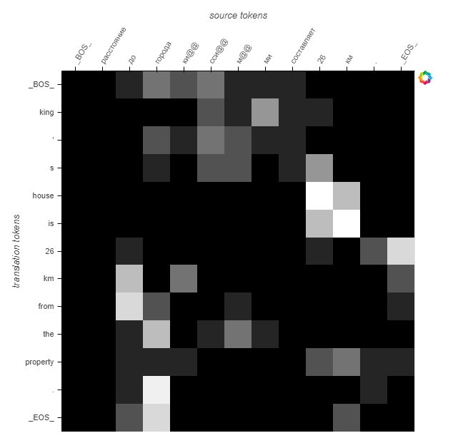 This sample is different, because of the rare words.
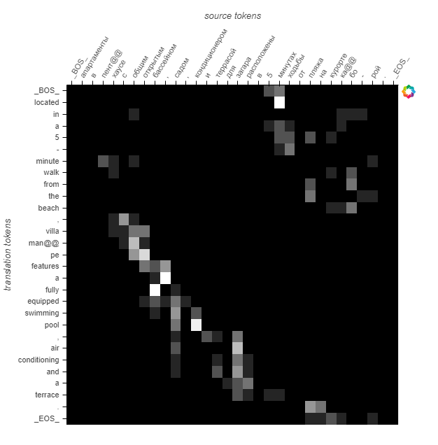 This sample is also different, because of rare words.
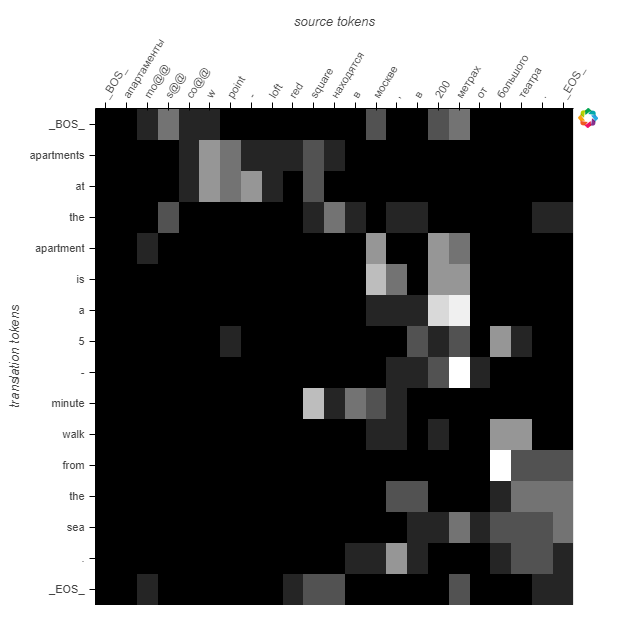 This sample is more difficult to interpret. There are rare words plus numbers and maybe abbreviotions.

